Valor Universal ODB++ Viewer Software (Free)

Download: Valor Universal ODB++ Viewer Software (Free)

RF Basics

Frequency

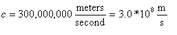
Frequency ဆိုတာ RF(Radio Frequency) တစ္ခုလံုးရဲ႕ အေျခခံအက်ဆံုး အစိတ္အပိုင္းျဖစ္တယ္။ Microwave Theory ပိုင္းမွာလည္း Frequency တန္းဖိုးက အေရၾကီးျပီး ရွဳပ္ေထြးလြန္းတဲ့ တြက္ခ်က္မွဳေတြမွာ အျမဲေနရာယူေနတာပါ။ Frequency ဆိုတာနဲ႕ sin wave နဲ႕ cosine wave ေတြကို သတိရၾကမယ္ထင္ပါတယ္။

Electromagnetic (EM) Wave

Electronic Wave အေၾကာင္းေျပာၿပီးဆို Magnetic Wave က ေနာက္က ဆက္ပါလာတာပါ။ Electronic wave သည္ Magnetic wave ႏွင့္ ေထာ့င္မွန္က် သည္။ ေအာက္ကပံုကေတာ့ sine wave ကို EM wave အေနနဲ႕ ျပထားတာပါ။

Radiation Pattern

Radiation Pattern ဆိုတာ Antenna ကေန ထုတ္လြတ္လိုက္တဲ့ Power ကို ေဖာ္ျပသည္လို႕ အဓိပၸါယ္ မွတ္ယူႏိုင္သည္။ Radiation Pattern ရဲ႕ ပံုက ပန္းသီးတစ္လံုးရဲ႕ပံုနဲ႕ တူတယ္။ အလယ္ဝင္ရိုးကို EM Wave လံုးဝမလြတ္ထုတ္ႏိုင္တဲ့ Null Location လို႕ေခၚျပီး အဲဒီ Null မ်ဥ္းေပၚမွာရွိတဲ့ ဘယ္ Receiver မဆို Transmitter က လြတ္တဲ့ သတင္းအခ်က္အလက္ေတြကို ရရွိမည္မဟုတ္။

Field Regions

Field Regions ၃ ခုရွိတယ္။

1. Far Field (Fraunhofer) Region
2. Reactive Near Field Region
3. Radiating Near Field (Fresnel) Region

Far Field (Fraunhofer) Region

Far Field Region က အေရးအၾကီးဆံုးျဖစ္သည္။ Antenna ရဲ႕ Radiation Pattern ကို Far Field Region နဲ႕ပဲ အဓိပၸါယ္ဖြင့္ဆိုသည္။ Antenna အလုပ္လုပ္တဲ့ Region လို႕ သတ္မွတ္လို႕ရပါသည္။ Far Field Region ျဖစ္ဖို႕ အခ်က္ ၃ ခ်က္နဲ႕ ျပည့္စံုရပါမယ္။

where; R = Far Field Region, D = Dimension of antenna

">>" ဆိုတာ အရမ္းၾကီးရမယ္လို႕ အဓိပၸါယ္ရတယ္။ အနည္းဆံုး ၁ဝ ဆၾကီးရပါမယ္။

Reactive Near Field Region 

Reactive Near Field Region ဆိုတာက Antenna ပါတ္ဝန္းက်င္က ေနရာေတြကို ဆိုလိုသည္။ Near Field Region ကို ေအာက္ပါအတိုင္းတြက္ခ်က္ႏိုင္သည္။

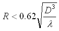
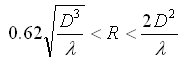
Radiating Near Field (Fresnel) Region

Radiation Near Field Region ကေတာ့ Far Field (Fraunhofer) Region နဲ႕ Reactive Near Field Region ၾကားမွာ ရွိပါသည္။ Radiation Near Field Region ကို ေအာက္ပါအတိုင္းတြက္ခ်က္ႏိုင္သည္။

Digital Transmitter Measurement

Objective

To understand

1. Characterization of IQ modulator: the Carrier Leakage and Sideband Suppression
2. The 1dB-Compression Point of a Transmitter. 
3. The output 3rd Order Intercept Point (OIP3) of a transmitter.
4. Modulation Analysis: Channel Power, ACPR,EVM

Characterization of IQ modulator: the Carrier Leakage and Sideband Suppression

A common approach to characterize the I-Q modulator performance is to apply two signals V sin(wt) and Vcos(wt) to the I and Q input terminals and examine the spectrum produced at the RF output.  In the ideal case, the output in the band of interest is simply given by;

• In practice, there are imbalances in the device (For example, gain and phase imbalance in the mixers and phase shifter network).

• Carrier leakage in a function of DC offset.
• It can be shown that the sideband suppression is a function of G & Φ.
  

1dB Compression Point

• The point at which the output power differs from the ideal transfer function by 1dB as the input power increases.

Dynamic Range

• The input power range over which the receiver provides a useful output. The low power limit is the sensitivity specification and upper limit is the input power at 1dB compression point.

Dynamic Range = Input 1dB Compression Point - Sensitivity Level

Output 3rd Order Intercept Point (OIP3)

IP3 can be calculated without extrapolation using above formula.

Modulation Analysis: Channel Power, ACPR, EVM, CCDF

Channel Power: Channel power is the average power in the frequency bandwidth of the signal of interest.  The measurement is generally defined as power integrated over the frequency band of interest.

ACPR: The adjacent Channel Power Ratio (ACPR) is usually defined as the ratio of the average power in the adjacent frequency channel to the average power in the transmitted channel.

EVM: The error vector is the vector difference at a given time between the ideal reference signal and the measured signal.  The error vector is a complex quantity that contains a magnitude and a phase component.  Error Vector Magnitude (EVM) is the root-mean-square (RMS) value of the error vector over time at the instants of the symbol clock transitions.

CCDF: The CCDF curve shows the probability that the power is equal to or above a certain peak-to-average ratio.  Figure A shows the power versus time plot.  This plot represents the instantaneous envelope power of the waveform.  Figure B displays the CCDF curve of the signal.  Here the x-axis is scaled to dB above the average signal power, which means we are actually measuring the peak-to-average ratios as opposed to absolute power levels.  The y-axis is the percent of time the signal spends at or above the power level specified by the x-axis.  For example, at t=1% on the y-axis, the corresponding peak-to-average ratio is 7.5dB onthe x-axis.

To be continued....

Virtual Router - Wifi Hot Spot for Windows 8, Windows 7 and 2008 R2

Virtual Router turns any Windows 7, Windows 8 or 2008 R2 computer into a Wifi Hot Spot using Windows' Wireless Hosted Network (Virtual Wifi) technology.

Where can Virtual Router be used?

Anywhere you are!

• Home
• Office
• School
• Airport
• Bus Station
• The Park
• Grandmas House
• The In-Laws
• Absolutely Anywhere!

Download @ http://virtualrouter.codeplex.com/

Explain how the length of the antennas, the transmit power and receiver sensitivity can have an impact on your CPE wireless coverage?

Antenna

The length of antenna is defined by the wavelength of the frequency. The longer length of antenna, the higher the gain of the antenna in dBi and the better coverage of CPE.

Transmit Power

Transmit Power is an important parameter of wireless design.

The higher transmit power at lower EVM can give a better performance and longer range of wireless coverage.

Sensitivity

Received Sensitivity is to measure the minimum received signal level of CPE.

Greater sensitivity = longer range

As the signal propagates away from the transmitter, the power density of the signal decreases, making it more difficult for a receiver to detect the signal as the distance increases. Improving the sensitivity on the receiver (making it more negative) will allow the radio to detect weaker signals, and can dramatically increase the transmission range.

Sensitivity, 1dB Compression Point and Dynamic Range

Sensitivity

• The smallest RF Signal that can produce a useful baseband signal at the receiver output.
• Determine how far the receiver can be from the transmitter and still receive an understandable message.

1dB Compression Point

• The point at which the output power differs from the ideal transfer function by 1dB as the input power increases.

Dynamic Range

• The input power range over which the receiver provides a useful output. The low power limit is the sensitivity specification and upper limit is the input power at 1dB compression point.

Dynamic Range = Input 1dB Compression Point - Sensitivity Level